Mapping and Binning a Metagenome Assembly¶

Downloading data¶

Now, go to a new directory and grab the data:

mkdir ~/mapping
cd ~/mapping

curl -O https://s3-us-west-1.amazonaws.com/dib-training.ucdavis.edu/metagenomics-scripps-2016-10-12/SRR1976948.abundtrim.subset.pe.fq.gz
curl -O https://s3-us-west-1.amazonaws.com/dib-training.ucdavis.edu/metagenomics-scripps-2016-10-12/SRR1977249.abundtrim.subset.pe.fq.gz

And extract the files:

for file in *fq.gz
  do
  gunzip $file
done

We will also need the assembly; rather than rebuilding it, you can download a copy that we saved for you:

curl -O https://s3-us-west-1.amazonaws.com/dib-training.ucdavis.edu/metagenomics-scripps-2016-10-12/subset_assembly.fa.gz
gunzip subset_assembly.fa.gz

Optional: look at tetramer clustering¶

The mapping is going to take a while, so while it’s running we can look at the tetramer nucleotide frequencies of all of our assembled contigs. For that, we’ll need this notebook:

cd ~/
curl -O https://raw.githubusercontent.com/ngs-docs/2017-ucsc-metagenomics/master/files/sourmash_tetramer.ipynb
cd -

and during the mapping we’ll load this notebook in the Jupyter notebook console. Note, the address of that will be:

echo http://$(hostname):8000/

...back to mapping!

Mapping the reads¶

First, we will need to to index the megahit assembly:

bwa index subset_assembly.fa

Now, we can map the reads:

for i in *fq
  do
      bwa mem -p subset_assembly.fa $i > ${i}.aln.sam
  done

Converting to BAM to quickly quantify¶

First, index the assembly for samtools:

samtools faidx subset_assembly.fa

Then, convert both SAM files to BAM files:

for i in *.sam
  do
    samtools import subset_assembly.fa $i $i.bam
    samtools sort $i.bam $i.bam.sorted
    samtools index $i.bam.sorted.bam
  done

Now we can quickly get a rough count of the total number of reads mapping to each contig using samtools:

for i in *sorted.bam
  do
    samtools idxstats $i > $i.idxstats
    cut -f1,3 $i.idxstats > $i.counts
  done

Binning the assembly¶

Finally, run the MaxBin! Note: MaxBin can take a lot of time to run and bin your metagenome. As this is a workshop, we are doing three things that sacrifice quality for speed.

1. We are only using 2 of the 6 datasets that were generated for the this project. Most binning software, including MaxBin, rely upon many samples to accurately bin data. And, we have subsampled the data to make it faster to proess.
2. We did quick and dirty contig estimation using samtools. If you use MaxBin, I would recommend allowing them to generate the abudance tables using Bowtie2. But, again, this will add to the run time.
3. We are limiting the number of iterations that are performed through their expectation-maximization algorithm (5 iterations instead of 50+). This will likely limit the quality of the bins we get out. So, users beware and read the user’s manual before proceeding with your own data analysis.

First, we will get a list of the count files that we have to pass to MaxBin:

cd ~/mapping
mkdir binning
cd binning
ls ../*counts > abundance.list

Now, on to the actual binning:

run_MaxBin.pl -contig ../subset_assembly.fa -abund_list abundance.list -max_iteration 5 -out mbin

This will generate a series of files. Take a look at the files generated. In particular you should see a series of *.fasta files preceeded by numbers. These are the different genome bins predicted by MaxBin.

Take a look at the mbin.summary file. What is shown?

Now, we are going to generate a concatenated file that contains all of our genome bins put together. We will change the fasta header name to include the bin number so that we can tell them apart later.

for file in mbin.*.fasta
  do
    num=${file//[!0-9]/}
    sed -e "/^>/ s/$/ ${num}/" mbin.$num.fasta >> binned.concat.fasta
  done

And finally make an annotation file for visualization:

echo label > annotation.list
grep ">" binned.concat.fasta |cut -f2 -d ' '>> annotation.list

Visualizing the bins¶

Now that we have our binned data there are several different things we can do. One thing we might want to do is check the quality of the binning– a useful tool for this is CheckM. We can also visualize the bins that we just generated using VizBin.

First, install VizBin:

cd
sudo apt-get install libatlas3-base libopenblas-base
curl -L https://github.com/claczny/VizBin/blob/master/VizBin-dist.jar?raw=true > VizBin-dist.jar

VizBin can run in OSX or Linux but is very hard to install on Windows. To simplify things we are going to run VizBin in the desktop emulator through JetStream (which is ... a bit clunky). So, go back to the Jetstream and open up the web desktop simulator.

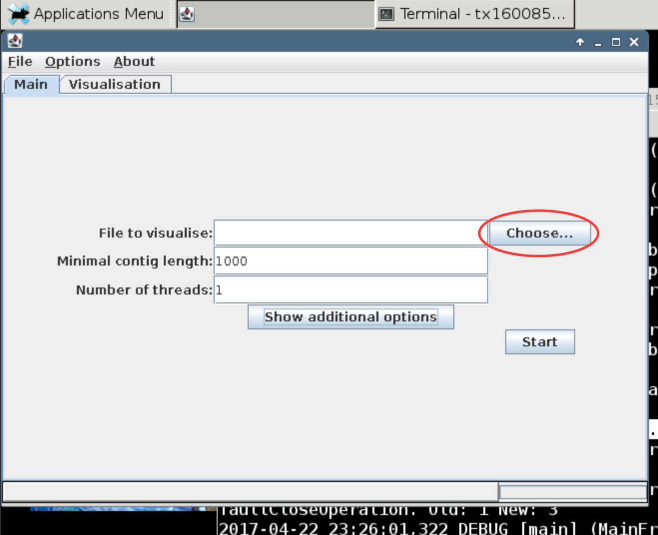
Open the terminal through the desktop simulator and open VizBin:

java -jar VizBin-dist.jar

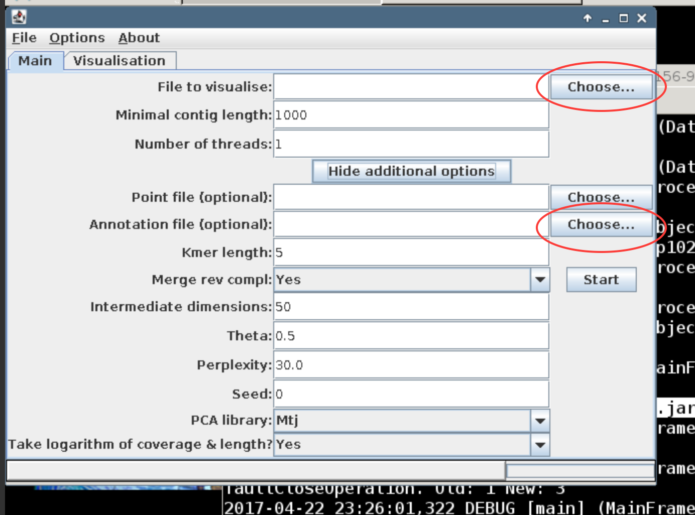
This should prompt VizBin to open in another window. Click the choose button to open file browser to navigate to the binning folder (~/mapping/binning). There you will find the concatenated binned fasta file (binned.concat.fasta). Upload this file and hit run.

What do you see? Read up a bit on VizBin to see how the visualization is generated.

Now, upload the annotation.list file as an annotation file to VizBin. The annotation file contains the bin id for each of the contigs in the assembly that were binned.

How do the two binning methods look in comparison?

Now we will search and compare our data.